FINN is an R-package of a forest gap model that is designed to be fit to data and integrates with neural networks. The package provides various functions that allow the user to customize the model from a mechanistic forest gap model to a mostly data-driven neural network. Individual processes can be replaced by neural networks and custom functions can be incorporated, or a combination of both. The package contains the FINN model itself and provides the tools to specify, modify, and calibrate different configurations of FINN. It also provides functions to simulate under any environmental conditions to which FINN was calibrated and to analyse learned processes via xAI (Accumulated Local Effect Plots )
How FINN works
FINN simulated forests with discrete time steps. Its state is a set of cohorts (groups of same-species, same-size trees) described by their size, species, and number. At each time step four demographic processes act on that state: competition for light, growth, mortality, and regeneration. The updated cohorts become the state for the next step. For each step stand-level variables DBH, basal area, tree numbers, and demographic rates are recorded and provided as simulation output.
What separates FINN from other DVM is that each process can be a mechanistic function, a neural network, or a mixture of the two, and all of them are calibrated together by gradient descent. Each response is combined in a joint likelihood that consists of a Gaussian for growth, a binomial for mortality, a negative binomial for regeneration.
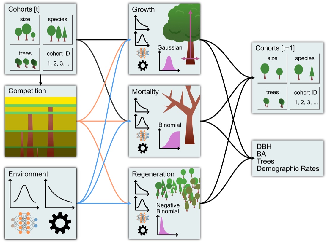
FINN’s structure. Each timestep, the current cohorts (their size, species and number) pass through the four demographic processes (competition, growth, mortality and regeneration) to produce the next cohorts and the stand-level outputs (DBH, basal area, tree numbers, demographic rates). The environment feeds growth, mortality and regeneration; each of those processes can be a mechanistic function, a neural network, or both (gear / network icons), and each is fit with its own likelihood (Gaussian for growth, binomial for mortality, negative binomial for regeneration). Figure from Käber & Pichler (2026).
This vignette builds a fully mechanistic model from known parameters and simulates it to showcase a key functionality of FINN: fitting a full DVM to recover (unknown) processes. Two later vignettes provide example on how to fit FINN to real forest inventory data: Fitting FINN to forest inventory data calibrates a model to real data and replaces the growth process with a neural network, another vignette on Mortality does the same for mortality. If you want to learn how a hybrid Dynamic Vegetation Model looks like and how you can build your own for inference and prediction FINN is the right tool and these vignettes will show you how to do it.
Installation
Install the released version of FINN from CRAN:
install.packages("FINN")Or the development version from GitHub. If you encounter problems running the code or understanding the documentation, please let us know by opening an issue on the GitHub repository.
# install.packages("devtools")
devtools::install_github("FINNverse/FINN")
Run the model
Load the package and setup some basic simulation parameters.
library(FINN)
library(data.table)
library(ggplot2)

Ntimesteps = 500  # number of timesteps
Nsites = 1 # number of sites
patch_size = 0.1
Nsp = 5 # number of species
Species parameters
The user can specify the species parameters. For each process species parameters are stored in vectors or matrices with rows representing species and columns representing different parameters. There are two kinds of parameters 1) process parameters like light requirements and effect of size (DBH) on a process. 2) Environmental parameters that modulate the effect of the environment on a process. Environmental parameters can be related to the processes with R formulas and naturally provide you with the option to include an intercept that modulates the overall effect size of a process.
The following code sets up a simple model with five species and one environmental variable. Some species parameters are hand-picked to span a range of demographic strategies and some are drawn at random: the exact numbers are arbitrary, chosen only to provide a set of species with different demographic roles in succession. In a real application you would not set them at all; they would be learned from data (see the Fitting FINN to forest inventory data vignette). However, this kind of flexibility also provides you with the opportunity to explore the sensitivity of the model quire easily.
FINN.seed(1234)
# we draw the same shade parameters for each process for simplicity
# shade parameters correspond to the fraction of light a species needs to successfully grow, regenerate, or survive.
shadeSP = c(0.1,0.2,0.5,0.5,0.7)

# regeneration parameters
parReg = shadeSP # regeneration is only dependent on shade and environment
parRegEnv = matrix(c(
  c(1,2,3,3,5), # intercept regulating the overall effect size
  runif(Nsp, -2, 2) # the second parameter modulates the effect of the environmental variable
  ),Nsp, 2)

# growth parameters
parGrowth = matrix(c(
  shadeSP, # see above
  c(0.04,0.05,0.05,0.06,0.1) # the second growth parameter modulates the size dependent growth
  ),Nsp, 2)

parGrowthEnv = matrix(c(
  c(0.2,0.3,0.5,1,1)*0.5, # intercept regulating the overall effect size
  runif(Nsp, -2, -0.5) # the second parameter modulates the effect of the environmental variable
  ),Nsp, 2)

# mortality parameters
parMort = matrix(c(
  as.numeric(scale(shadeSP)), # see above
  as.numeric(scale(parGrowth[,2])), # the second growth parameter modulates the size dependent mortality
  rep(0,Nsp) # the third mort parameter modulates the growth dependent mortality
  ),Nsp, 3)
parMortEnv = matrix(c(
  runif(Nsp, -3, -2), # intercept regulating the overall effect size
  runif(Nsp, -3, -2) # the second parameter modulates the effect of the environmental variable
  ), Nsp, 2)

# allometric parameters for the calculation of tree height from a trees diameter
parComp = matrix(c(
  c(0.5,0.5,0.4,0.7,0.6), # parHeight
  c(0.3,0.2,0.2,0.2,0.1) # Competition strength
),Nsp, 2)

# Create a wide-format data.table with one row per species
pars_dt <- data.table(
  speciesID   = 1:Nsp,
  reg         = parReg,
  growth1      = parGrowth[, 1],
  growth2      = parGrowth[, 2],
  mort1        = parMort[, 1],
  mort2        = parMort[, 2],
  mort3        = parMort[, 3],
  compHeight  = parComp[, 1],
  compStrength= parComp[, 2],
  regEnv1     = parRegEnv[, 1],
  regEnv2     = parRegEnv[, 2],
  growthEnv1  = parGrowthEnv[, 1],
  growthEnv2  = parGrowthEnv[, 2],
  mortEnv1    = parMortEnv[, 1],
  mortEnv2    = parMortEnv[, 2]
)
pars_dt
#>    speciesID   reg growth1 growth2      mort1         mort2 mort3 compHeight
#>        <int> <num>   <num>   <num>      <num>         <num> <num>      <num>
#> 1:         1   0.1     0.1    0.04 -1.2247449 -8.528029e-01     0        0.5
#> 2:         2   0.2     0.2    0.05 -0.8164966 -4.264014e-01     0        0.5
#> 3:         3   0.5     0.5    0.05  0.4082483 -4.264014e-01     0        0.4
#> 4:         4   0.5     0.5    0.06  0.4082483 -5.917509e-16     0        0.7
#> 5:         5   0.7     0.7    0.10  1.2247449  1.705606e+00     0        0.6
#>    compStrength regEnv1    regEnv2 growthEnv1 growthEnv2  mortEnv1  mortEnv2
#>           <num>   <num>      <num>      <num>      <num>     <num>     <num>
#> 1:          0.3       1 -1.5451864       0.10  -1.039534 -2.306409 -2.162704
#> 2:          0.2       2  0.4891976       0.15  -1.985756 -2.455025 -2.713777
#> 3:          0.2       3  0.4370989       0.25  -1.651174 -2.717266 -2.733179
#> 4:          0.2       3  0.4935178       0.50  -1.000874 -2.076567 -2.813277
#> 5:          0.1       5  1.4436615       0.50  -1.228623 -2.707684 -2.767774
Two conventions in that code are worth explaining:
-
Why the environmental parameters are a
matrix. Each row is a species and the two columns are the[intercept, slope]of the linear effect of the one environmental variable. Internally FINN represents an environmental effect as a neural network, so it actually stores a list of weight matrices; for a plain linear term that list has a single entry, andcreateProcess()wraps a bare matrix for you. That is why the sameinitEnvslot also accepts a full network; when a process is replaced by one, the slot simply holds more weight matrices and the interface does not change. -
Why the mortality parameters use
scale(). These are arbitrary illustrative values. In the mortality function the first two parameters act as coefficients (they multiply light and size inside a link function), rather than as the light thresholds thatshadeSPrepresents for growth and regeneration.scale()centres them and gives them unit variance, which keeps the resulting mortality rates in a plausible range for this synthetic example. For a real fit you would not set these by hand at all; they are learned.
Environment and disturbances
Next we have to specify the environmental input variables. These variables are used to calculate the effect of the environment on the processes. The environmental variables are supplied with a data.frame/data.table in a long format with the columns siteID and year and the environmental variables as additional columns.
# we first generate a data.table with all combinations of site and timestep.
env_dt <- data.table(
  expand.grid(
    list(
      siteID = 1:Nsites,
      year = 1:Ntimesteps
    )
  )
)

dist_dt <- env_dt

# for this very simple model we will have a constant environment for all sites and timesteps
env_dt$env1 = rep(0, Ntimesteps)

# Disturbances are optional and specified per site-year, as a single number:
# the fraction of patches destroyed that year (0 = nothing happens).
#
# Here a disturbance strikes independently each year with probability 5%
# (a Bernoulli draw), and when it does it removes 50-100% of the patches
# (a uniform intensity). No disturbance in a year leaves the value at 0.
disturbance_frequency = 0.05
n <- Ntimesteps * Nsites
dist_dt$intensity <- rbinom(n, 1, disturbance_frequency) * runif(n, 0.5, 1)
Simulate
The model can be run with the simulateForest function.
Its main arguments are model the assembled FINN model
(which already contains the processes), env the
environmental input data.table, and patches the number of
patches. Optionally disturbances
A model is assembled with finn(), which takes one
process per demographic component. Each process is built with
createProcess(), so the pattern is always
finn(growth_process = createProcess(...), mortality_process = createProcess(...), ...),
as in the call below.
The processes are specified with the createProcess
function. The first argument is a formula that specifies the relation
between environment and the process. The formula includes the intercept
and the environmental variables that are provided with env.
The second argument is the function that should be used for the process.
FINN includes the default functions growth,
mortality, and regeneration. The user can also
provide custom functions. The function should take the species
parameters and the environmental parameters as arguments. The third and
fourth arguments are the initial species and environmental
parameters.
Disturbances can be specified with the disturbance
argument, which requires a data.table with the columns siteID, year, and
intensity. The intensity is the fraction of patches that are disturbed
at that timestep.
The effect of environmental variable supplied with the environmental
data can be defined in the process functions. For example
~ 1 + env1 specifies an intercept and a linear effect of
env1. Both, the intercept 1 and the effect of
env1 can be modulated by the species parameters that were
specified above.
predictions <- list()
simulationModel = finn(N_species = Nsp,
  competition_process = createProcess(~0, func = FINN::competition),
  growth_process = createProcess(~1+env1, initEnv = parGrowthEnv,initSpecies = parGrowth, func = FINN::growth),
  regeneration_process = createProcess(~1+env1, initEnv = parRegEnv,initSpecies = parReg, func = FINN::regeneration),
  mortality_process = createProcess(~1+env1, initEnv = parMortEnv,initSpecies = parMort, func = FINN::mortality),
)

predictions[["patches_1"]] =
  simulateForest(simulationModel, init_cohort = NULL, env = env_dt, disturbance = dist_dt, device = "cpu", patches = 1)

simulationModel = finn(N_species = Nsp,
  competition_process = createProcess(~0, func = FINN::competition),
  growth_process = createProcess(~1+env1, initEnv = parGrowthEnv,initSpecies = parGrowth, func = FINN::growth),
  regeneration_process = createProcess(~1+env1, initEnv = parRegEnv,initSpecies = parReg, func = FINN::regeneration),
  mortality_process = createProcess(~1+env1, initEnv = parMortEnv,initSpecies = parMort, func = FINN::mortality),
)

predictions[["patches_100"]] =
  simulateForest(simulationModel, init_cohort = NULL, env = env_dt, disturbance = dist_dt, device = "cpu", patches = 100)
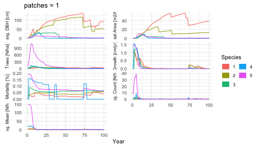
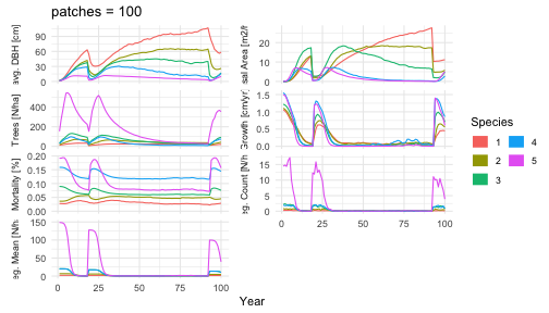
Naturally forest gap models are stochastic, so one patch is only one noisy realisation. Averaging over many patches creates a smooth stand-level aggregation of the forest state.
Aggregation of patches is done internally. simulateForest() returns patch-averaged, stand-level results in site. The mean() in the plotting code below only collapses the site dimension, which matters when you simulate more than one site.
If you need more than the stand-level averages, set return_cohorts to keep the raw per-cohort state for the timesteps you choose. This records each cohort’s size, species and tree number together with its growth and mortality rates. Use TRUE for every step, “last” for the final one, or a vector of timesteps such as c(1, 250, 500). Those come back in cohort and cohort. It is FALSE by default because storing every cohort at every timestep is expensive.
for(i in c("patches_1", "patches_100")){
  # $long$site is already averaged over patches; this mean() collapses sites
  p_dat <- predictions[[i]]$long$site[, .(value = mean(value)), by = .(year, species, variable)]
  p_dat[, variable2 := factor(
    variable,
    levels = c("dbh", "ba", "trees", "AL", "growth", "mort", "reg", "r_mean_ha"),
    labels =  c("avg. DBH [cm]", "Basal Area [m2/ha]", "Trees [N/ha]",
                "Available Light [%]", "Growth [cm/yr]", "Mortality [%]",
                "Reg. Count [N/ha]", "Reg. Mean [N/ha]")
    ),]
  p_dat[variable %in% c("ba", "trees"), value := value/patch_size,]
  p <- ggplot(p_dat[year <= 100], aes(x = year, y = value, color = factor(species))) +
  geom_line() +
  theme_minimal() +
  labs(x = "Year", y = "Value") +
  coord_cartesian(ylim = c(0, NA)) +
  facet_wrap(~variable2, scales = "free_y", ncol = 2, strip.position = "left") +
  theme(
    axis.title.y = element_blank(),
    strip.placement = "outside",
    strip.text.y.left = element_text(angle = 90)
  ) +
  guides(color = guide_legend(title = "Species", override.aes = list(linewidth = 5), ncol = 2, title.position = "top")) +
  scale_color_discrete(name = "Species") +
  ggtitle(paste0("patches = ",gsub("patches_", "", i)))

  print(p)
}
sessionInfo()
#> R version 4.5.0 (2025-04-11)
#> Platform: aarch64-apple-darwin20
#> Running under: macOS 26.5.1
#>
#> Matrix products: default
#> BLAS:   /Library/Frameworks/R.framework/Versions/4.5-arm64/Resources/lib/libRblas.0.dylib
#> LAPACK: /Library/Frameworks/R.framework/Versions/4.5-arm64/Resources/lib/libRlapack.dylib;  LAPACK version 3.12.1
#>
#> locale:
#> [1] C
#>
#> time zone: Europe/Berlin
#> tzcode source: internal
#>
#> attached base packages:
#> [1] stats     graphics  grDevices utils     datasets  methods   base
#>
#> other attached packages:
#> [1] ggplot2_3.5.2     data.table_1.17.8 FINN_0.1.0
#>
#> loaded via a namespace (and not attached):
#>  [1] vctrs_0.6.5        cli_3.6.6          knitr_1.50         rlang_1.2.0
#>  [5] xfun_0.57          processx_3.8.6     generics_0.1.4     torch_0.15.1
#>  [9] coro_1.1.0         labeling_0.4.3     glue_1.8.0         bit_4.6.0
#> [13] ps_1.9.1           scales_1.4.0       grid_4.5.0         abind_1.4-8
#> [17] evaluate_1.0.5     tibble_3.3.0       lifecycle_1.0.5    compiler_4.5.0
#> [21] dplyr_1.1.4        RColorBrewer_1.1-3 Rcpp_1.1.0         pkgconfig_2.0.3
#> [25] farver_2.1.2       R6_2.6.1           tidyselect_1.2.1   pillar_1.11.0
#> [29] callr_3.7.6        magrittr_2.0.3     withr_3.0.2        tools_4.5.0
#> [33] bit64_4.6.0-1      gtable_0.3.6