Fitting FINN to forest inventory data (Oregon, US FIA)
Source:vignettes/D-Fit_to_FIA.Rmd
D-Fit_to_FIA.RmdDynamic forest models are usually developed through a combination of encoding ecological knowledge into model structures and parameters. Usually the resulting parameters are then further refined by manual calibration procedures. Here we calibrate FINN directly from data: a subset of the US Forest Inventory & Analysis (FIA) program for Oregon, prepared exactly as in the Preparing your data for FINN vignette.
We fit FINN to 200 sites and evaluate on 200 held-out sites.
The calibration of the model for all species parameters relies on the
a torch backend and therefor takes several minutes, the vignette is
precompiled: vignettes/build.R knits
D-Fit_to_FIA.Rmd.orig once on a developer machine and
commits the resulting static .Rmd. So the code you see is
exactly the code that produced the output, and the package builds
anywhere without torch.
library(FINN)
library(torch)
library(data.table)
library(ggplot2)

# Training length. 500 is comfortably past convergence: every response plateaus
# by ~epoch 400 (checked across 3 seeds). Raising it changes nothing except the
# knit time.
EPOCHS <- 500L
The data
The input tables are built by
dev/make_extdata.R, which draws 400 sites
from the full Oregon FIA set in data-raw/ and splits them
into two train and test data. The climate
(fia_env_dt.csv) was created in the FINN-fia analysis repo
(scripts/03_attach_environment.R →
07_prepare_finn_inputs.R); see
data-raw/README.md for the full chain.
The data consists of 200 sites to fit on, and 200 holdout sites for evaluation. A fitted FINN model should generalize to other sites. So the holdout is a genuine out-of-sample test.
ext <- function(f) system.file("extdata", f, package = "FINN")

# --- training sites --------------------------------------------------------
obs_dt     <- fread(ext("fia_obs_dt.csv"))     # observations, wide (one column per variable)
env_dt     <- fread(ext("fia_env_dt.csv"))     # RAW, untransformed climate
init_trees <- fread(ext("fia_init_trees.csv"))
species_dt <- fread(ext("fia_species_dt.csv"))

# --- holdout sites: never seen during fitting ------------------------------
obs_test   <- fread(ext("fia_obs_test.csv"))
env_test   <- fread(ext("fia_env_test.csv"))
init_test  <- fread(ext("fia_init_test.csv"))

# long form of the observations, so later we can match FINN's long predictions
# (sim$long$site) with a single merge()
resp  <- c("dbh", "ba", "trees", "growth", "mort", "reg")
to_long <- function(d) melt(d, id.vars = c("siteID", "year", "species", "species_name"),
                            measure.vars = resp, variable.name = "variable", value.name = "obs")
obs_long  <- to_long(obs_dt)
test_long <- to_long(obs_test)

cat(sprintf("train: %d sites | holdout: %d sites | %d species | years %s\n",
            uniqueN(obs_dt$siteID), uniqueN(obs_test$siteID), uniqueN(obs_dt$species),
            paste(sort(unique(obs_dt$year)), collapse = " & ")))
#> train: 200 sites | holdout: 200 sites | 11 species | years 1 & 2
species_dt
#>     species            species_name
#>       <int>                  <char>
#>  1:       1   Pseudotsuga menziesii
#>  2:       2         Pinus ponderosa
#>  3:       3          Pinus contorta
#>  4:       4          Abies concolor
#>  5:       5           Abies grandis
#>  6:       6      Tsuga heterophylla
#>  7:       7       Tsuga mertensiana
#>  8:       8 Lithocarpus densiflorus
#>  9:       9             Alnus rubra
#> 10:      10          Abies amabilis
#> 11:      11                   other
The environment is supplied in natural units: with
env_autoscale = TRUE (the default) FINN z-standardizes the
predictors internally and reuses the same constants at prediction time,
so raw values are all we ever pass.
ggplot(melt(env_dt[, c("temp", "prec")], measure.vars = c("temp", "prec")),
       aes(value)) +
  geom_histogram(bins = 20, fill = "grey40") +
  facet_wrap(~variable, scales = "free", labeller = as_labeller(
    c(temp = "Mean~annual~temp~(degree*C)", prec = "Annual~precip~(mm)"), label_parsed)) +
  labs(x = NULL, y = "site x year") + theme_minimal()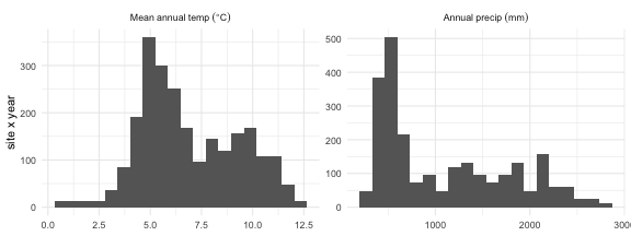
Stand abundance, measured as total basal area per plot (summed over species), against the temperature and precipitation gradients:
# total stand basal area per plot: sum over species, averaged over inventories
site_ba  <- obs_dt[, .(ba = sum(ba, na.rm = TRUE)), by = .(siteID, year)][
                   , .(ba = mean(ba)), by = siteID]
site_env <- env_dt[, .(temp = mean(temp), prec = mean(prec)), by = siteID]
grad <- melt(merge(site_ba, site_env, by = "siteID"),
             id.vars = c("siteID", "ba"), measure.vars = c("temp", "prec"),
             variable.name = "gradient")

ggplot(grad, aes(value, ba)) +
  geom_point(alpha = 0.4, size = 0.9, colour = "grey30") +
  geom_smooth(method = "loess", se = FALSE, colour = "firebrick", linewidth = 0.9) +
  facet_wrap(~gradient, scales = "free_x", labeller = as_labeller(
    c(temp = "Mean~annual~temp~(degree*C)", prec = "Annual~precip~(mm)"), label_parsed)) +
  labs(x = NULL, y = "Total basal area per plot") + theme_minimal()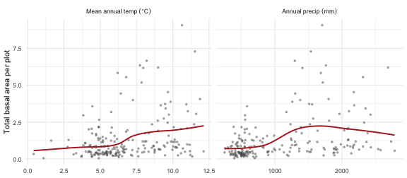
Initial cohorts
Each simulation starts from the observed first inventory. We build the starting state for both samples, the holdout gets its own cohorts, from its own sites.
Nsp <- max(obs_dt$species)
init_cohorts      <- makeInitCohorts(init_trees, Nspecies = Nsp)
init_cohorts_test <- makeInitCohorts(init_test,  Nspecies = Nsp)
# shared colours for the two model variants, reused by the scatter and ALE panels
model_cols <- c("Process (mechanistic)" = "#1b9e77", "Hybrid (growth = NN)" = "#d95f02")
Fit a Process-FINN
In the fully mechanistic configuration every process keeps its
predefined form, while its species and environmental parameters are
learned (optimize* = TRUE) and the formula chooses which
environmental predictors enter the growth, regeneration and mortality
responses. The model is calibrated end-to-end by gradient descent
through the entire simulation.
We pass two climate drivers rather than all six
available. ~. would use every column, but the six are
strongly collinear; temp and tempmin correlate
at r = 0.93, prec and precwarmq at 0.86, and
two principal components carry 90% of the variance. Collinear predictors
are not a problem for the fit (that is what ALE is designed
for), but they are a problem for the interpretation below: two
drivers that correlate at 0.93 have no separately identifiable response
curves, so calling each one a “niche” would be reading structure into an
arbitrary split. Two weakly-correlated drivers (r = 0.64) give curves
that mean what the text says they mean. Measured across three seeds, the
cost is nothing on growth (0.56 vs 0.55 held out) and ~0.02 on basal
area, tree numbers and regeneration.
FINN.seed(42)
m <- finn(
  N_species            = uniqueN(obs_dt$species),
  recruits_dbh         = 12.9,   # DBH (cm) assigned to a new recruit; ~ FIA's 12.7 cm (5 in) minimum
  competition_process  = createProcess(~0, FINN::competition,  optimizeSpecies = TRUE),
  growth_process       = createProcess(~ temp + prec, FINN::growth,       optimizeSpecies = TRUE, optimizeEnv = TRUE),
  regeneration_process = createProcess(~ temp + prec, FINN::regeneration, optimizeSpecies = TRUE, optimizeEnv = TRUE),
  mortality_process    = createProcess(~ temp + prec, FINN::mortality,    optimizeSpecies = TRUE, optimizeEnv = TRUE)
)
fit(m,
  env         = env_dt,      # raw climate
  data        = obs_dt,
  init_cohort = init_cohorts,
  device      = "cpu",
  epochs      = EPOCHS,
  batchsize   = 40L,
  patches     = 4,
  patch_size  = 0.06,
  lr          = 0.01,
  env_autoscale   = TRUE,        # default
  plot_progress   = FALSE        # the convergence plot below is the readable one
)
Replace growth with a neural network (Hybrid-FINN)
FINN’s defining feature is that any single demographic
process can be swapped from a mechanistic function to a neural
network, while the others stay mechanistic, a hybrid
model. The mechanistic processes keep the system ecologically
constrained; the network absorbs structure the fixed functional form
cannot express. Here we replace growth with a small
neural network via createHybrid(), leaving competition,
regeneration and mortality mechanistic, and refit on the same data with
the identical fit() call.
FINN.seed(42)
m_hybrid <- finn(
  N_species            = uniqueN(obs_dt$species),
  recruits_dbh         = 12.9,
  competition_process  = createProcess(~0, FINN::competition,  optimizeSpecies = TRUE),
  growth_process       = createHybrid(~ temp + prec, hidden = c(20L, 20L), transformer = FALSE),  # NN replaces growth
  regeneration_process = createProcess(~ temp + prec, FINN::regeneration, optimizeSpecies = TRUE, optimizeEnv = TRUE),
  mortality_process    = createProcess(~ temp + prec, FINN::mortality,    optimizeSpecies = TRUE, optimizeEnv = TRUE)
)
fit(m_hybrid,
  env = env_dt, data = obs_dt, init_cohort = init_cohorts, device = "cpu",
  epochs = EPOCHS, batchsize = 40L, patches = 4, patch_size = 0.06,
  lr = 0.01, env_autoscale = TRUE, plot_progress = FALSE
)
With both variants fitted, the rest of the vignette inspects and
compares them: training convergence, a summary() of the
learned structure, predicted-vs-observed fit, the learned niches, and
the accumulated local effects that reveal what the network learned.
Training convergence
Both variants are trained the same way. Because the losses are scaled
by their intercept-only baselines, m$history can be read
per response on one axis, and the dashed line at 1 is a
real reference: it is the intercept-only model, so a curve below it
means that response is predicted better than by its own mean.
hist_dt <- as.data.table(do.call(rbind, m$history))[, 1:6]
setnames(hist_dt, c("dbh", "ba", "trees", "growth", "mort", "reg"))
hist_dt[, epoch := .I]
ggplot(melt(hist_dt, id.vars = "epoch", variable.name = "response"),
       aes(epoch, value, colour = response)) +
  geom_hline(yintercept = 1, linetype = "dashed", colour = "grey40") +
  geom_line(alpha = 0.8) +
  scale_y_log10() +
  scale_colour_viridis_d() +
  labs(x = "epoch", y = "loss / intercept-only baseline\n(1 = no better than the mean)",
       colour = NULL) +
  theme_minimal()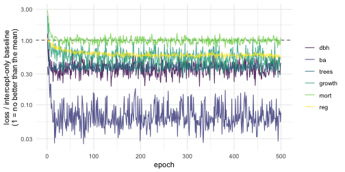
The structural responses drop well below 1 within a few epochs. The per-tree rates sit much closer to it; they are only weakly constrained by two inventories, which is the honest picture and the reason for the caveat further down.
What the model learned: summary()
summary() gives a compact overview of the learned
structure: for each process and species it reports how important
each environmental predictor is (ALE-variance importance,
rate-normalised) and its average conditional effect. It reuses the
cached conditional effects, so once ALE() (below) or a
previous summary() has run it needs no further
simulation.
summary(m)
FINN model summary
==================

### GROWTH

Analytical ALE importance (rate-normalised) (species in columns):
 variable    sp1    sp2      sp3      sp4      sp5   sp6   sp7    sp8   sp9
     temp 0.0242 0.0133 0.744175 0.000735 0.000385 0.473 0.489 2.7839 0.342
     prec 0.2288 2.5776 0.000987 0.005823 0.002549 0.297 0.383 0.0168 0.635
   sp10   sp11
 2.7389 0.0854
 0.0286 0.4186

Average conditional effects (mean; species in columns):
 variable     sp1     sp2     sp3      sp4      sp5    sp6    sp7      sp8
     temp -0.0158 0.00638 0.07445 -0.00308  0.00199 0.0975 0.0421 -0.03546
     prec  0.0497 0.08533 0.00361 -0.01113 -0.00454 0.0713 0.0354 -0.00381
     sp9    sp10    sp11
 -0.0879  0.2412 -0.0218
  0.1042 -0.0224  0.0496

### MORTALITY

Analytical ALE importance (rate-normalised) (species in columns):
 variable    sp1    sp2    sp3   sp4  sp5    sp6    sp7    sp8      sp9  sp10
     prec 0.0605 3.6817 0.4992 0.201 1.07 0.0711 0.5722 0.0183 0.292514 1.192
     temp 0.0508 0.0545 0.0836 0.200 0.41 1.9825 0.0238 1.5557 0.000331 0.237
   sp11
 0.0151
 0.3825

Average conditional effects (mean; species in columns):
 variable     sp1      sp2     sp3     sp4    sp5      sp6     sp7     sp8
     prec 0.00770  0.02773 0.02021 -0.0245 0.0262 -0.00244 -0.0976 -0.0102
     temp 0.00742 -0.00326 0.00883 -0.0211 0.0232 -0.01712  0.0149 -0.0645
       sp9    sp10    sp11
  0.009963 -0.0741 -0.0066
 -0.000322 -0.0302 -0.0297

### REGENERATION

Analytical ALE importance (rate-normalised) (species in columns):
 variable     sp1   sp2   sp3    sp4   sp5    sp6   sp7   sp8   sp9  sp10  sp11
     prec 0.00331 0.923 0.148 1.1918 0.337 1.0344 0.501 0.294 0.677 0.701 1.169
     temp 0.91140 0.144 0.564 0.0518 0.676 0.0754 0.860 0.452 0.423 0.360 0.132

Average conditional effects (mean; species in columns):
 variable   sp1    sp2   sp3    sp4    sp5   sp6    sp7     sp8   sp9   sp10
     prec 0.143 -3.083 -1.33 -0.410 -0.794 0.487  0.500 0.00812 0.543  1.074
     temp 2.604  0.766 -1.62  0.077 -0.644 0.125 -0.553 0.01056 0.389 -0.827
   sp11
  1.525
 -0.514
The niche and ALE sections below unpack this overview into per-driver response curves.
Assess the fit: in-sample and on held-out sites
The fit was calibrated on the 200 training sites, so scoring it there only tells us how well it reproduces them. The honest question is whether it transfers, so we simulate each model twice, once on the training sites, once on the 200 held-out sites, and score both with Spearman correlation (rank agreement) and RMSE (in each response’s own units), matched on site × year × species.
# One prediction pass per model x sample. The holdout is driven only by its own
# environment and starting cohorts; nothing about it entered the fit.
pred_of <- function(model, label, env, init, obs_l, split) {
  model$eval()                                   # deterministic: dropout off
  sim <- predict(model, env = env, init_cohort = init,
                 patches = 4, patch_size = 0.06, device = "cpu")
  merge(obs_l, sim$long$site, by = c("siteID", "year", "species", "variable"
  ))[, `:=`(model = label, split = split)][]
}
FINN.seed(1)
obs_pred <- rbind(
  pred_of(m,        "Process (mechanistic)", env_dt,   init_cohorts,      obs_long,  "train"),
  pred_of(m,        "Process (mechanistic)", env_test, init_cohorts_test, test_long, "holdout"),
  pred_of(m_hybrid, "Hybrid (growth = NN)",  env_dt,   init_cohorts,      obs_long,  "train"),
  pred_of(m_hybrid, "Hybrid (growth = NN)",  env_test, init_cohorts_test, test_long, "holdout"))

metrics <- obs_pred[is.finite(obs) & is.finite(value),
                    .(spearman = round(cor(obs, value, method = "spearman"), 2),
                      rmse     = round(sqrt(mean((obs - value)^2)), 2),
                      n        = .N), by = .(model, split, variable)]

comparison <- dcast(metrics, variable + model ~ split, value.var = c("spearman", "rmse"))
setcolorder(comparison, c("variable", "model", "spearman_train", "spearman_holdout",
                          "rmse_train", "rmse_holdout"))
comparison[order(variable, model)]
#> Key: <variable, model>
#>     variable                 model spearman_train spearman_holdout rmse_train
#>       <fctr>                <char>          <num>            <num>      <num>
#>  1:      dbh  Hybrid (growth = NN)           0.80             0.73      13.05
#>  2:      dbh Process (mechanistic)           0.80             0.73      12.93
#>  3:       ba  Hybrid (growth = NN)           0.80             0.79       0.12
#>  4:       ba Process (mechanistic)           0.80             0.80       0.12
#>  5:    trees  Hybrid (growth = NN)           0.78             0.77       0.75
#>  6:    trees Process (mechanistic)           0.78             0.78       0.77
#>  7:   growth  Hybrid (growth = NN)           0.58             0.50       0.09
#>  8:   growth Process (mechanistic)           0.60             0.56       0.10
#>  9:     mort  Hybrid (growth = NN)           0.18             0.04       0.15
#> 10:     mort Process (mechanistic)           0.17             0.03       0.15
#> 11:      reg  Hybrid (growth = NN)           0.23             0.23       6.20
#> 12:      reg Process (mechanistic)           0.23             0.24       6.22
#>     rmse_holdout
#>            <num>
#>  1:        13.89
#>  2:        13.78
#>  3:         0.09
#>  4:         0.09
#>  5:         0.77
#>  6:         0.78
#>  7:         0.10
#>  8:         0.11
#>  9:         0.16
#> 10:         0.15
#> 11:         6.47
#> 12:         6.46
The structural variables (basal area, tree numbers and diameter) are reconstructed well, and hold up on sites the model never saw: that gap between the train and holdout columns is the part that matters, because it is the only evidence that the fitted processes generalise rather than memorise. The noisier per-tree rates (growth, mortality, regeneration) are harder to constrain from two inventories and should be read with that in mind (see the caveat below). The hybrid tracks the mechanistic model on the structural variables, with no growth equation specified, which is what makes hybrids useful when a process’s form is uncertain; the surrounding mechanistic processes still anchor the model ecologically.
# facet_wrap, NOT facet_grid: the three responses live on completely different
# scales (dbh ~150 cm, ba ~8 m2, trees ~20). facet_grid(scales = "free") frees x
# per column but y per ROW, so ba and trees would be drawn on dbh's y-axis -
# squashing them onto y = 0 and flattening the 1:1 line until a good fit looks
# like a broken one. facet_wrap frees both axes per panel.
ggplot(obs_pred[variable %in% c("dbh", "ba", "trees") & is.finite(obs)],
       aes(obs, value, colour = model)) +
  geom_abline(slope = 1, intercept = 0, colour = "grey40", linewidth = 0.3) +
  geom_point(alpha = 0.25, size = 0.5) +
  facet_wrap(~ split + variable, scales = "free", ncol = 3,
             labeller = labeller(.multi_line = FALSE)) +
  scale_colour_manual(values = model_cols) +
  labs(x = "observed", y = "predicted", colour = NULL) +
  theme_minimal() + theme(legend.position = "top")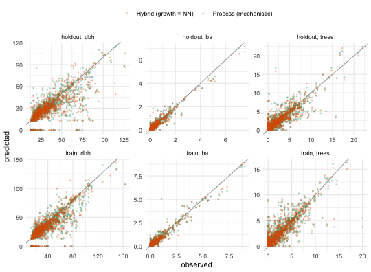
Each panel is on its own axes, and the grey line is 1:1, so the diagonal is the target in every panel regardless of the units on it.
A caveat on the rate variables.
growth,mortandregare per-tree rates and are only weakly constrained by two inventories, so their Spearman is a noisy estimate; refitting with a different random seed moves it by a few hundredths. Differences of that size between the models should not be over-read; the structural variables, estimated from far more information, are what carry the comparison.mortis the extreme case and gets a vignette of its own (Mortality: a binomial response and a neural-network process) because rank correlation is the wrong tool for a response that is mostly zeros.
Interpreting the growth process with ALE
ALE() returns the accumulated local
effect of every driver on each process, the effect measure of
choice when predictors are correlated, because it accumulates
local changes within the observed data instead of extrapolating
to unrealistic combinations. Running it on both fitted
models lets us read what growth responds to and compare the
mechanistic process with the neural-network hybrid, across growth’s
structural inputs (tree size, light) and its
environmental niche (climate). It returns one table per
process (growth, mortality,
regeneration); we use the growth table of each model.
FINN.seed(1)
ale_proc <- ALE(m,        env_dt, init_cohorts, plot = FALSE)   # mechanistic growth
ale_hyb  <- ALE(m_hybrid, env_dt, init_cohorts, plot = FALSE)   # growth = NN

# one tidy table with both variants. Environmental drivers come back on the
# model's scaled axis, so back-transform temp/prec to natural units (deg C, mm);
# the structural drivers (dbh, light) are already on their natural axes.
to_natural <- function(a, model) {
  sc <- as.data.table(model$env_scaling)[, .(var = variable, center, scale)]
  merge(data.table(a), sc, by = "var", all.x = TRUE)[!is.na(center), x := x * scale + center]
}
growth <- rbind(
  to_natural(ale_proc$growth, m)[,        model := "Process (mechanistic)"],
  to_natural(ale_hyb$growth,  m_hybrid)[, model := "Hybrid (growth = NN)"])
growth <- merge(growth, species_dt, by = "species")
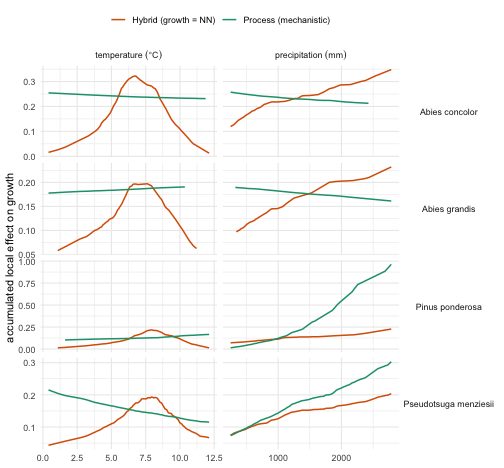
One helper plots the growth ALE of both variants for any set of drivers, one panel per species × driver, with independent axes so responses of very different magnitude stay legible side by side:
plot_growth_ale <- function(vars, labs) {
  d <- growth[var %in% vars & species %in% c(1, 2, 4, 5)]   # the four focal species
  d[, var := factor(var, levels = names(labs))]
  ggplot(d, aes(x, ale, colour = model)) +
    geom_line(linewidth = 0.7) +
    facet_grid(species_name ~ var, scales = "free",
               labeller = labeller(var = as_labeller(labs, label_parsed),
                                    species_name = label_value)) +
    scale_colour_manual(values = model_cols) +
    labs(x = NULL, y = "accumulated local effect on growth", colour = NULL) +
    theme_minimal() + theme(legend.position = "top", strip.text.y = element_text(angle = 0))
}
Environmental niches
Because the environmental responses are learned rather than prescribed, each curve is an inferred niche, how a species’ growth scales along a climate gradient. Growth generally rises with precipitation, and the temperature responses are single-peaked, with an optimum in the middle of the sampled range.
Read these as illustrations of what ALE recovers, not as settled ecology. The per-species shapes are noisier than the structural responses below; growth is weakly constrained by two inventories (see the caveat above), and the mechanistic and hybrid curves do not always agree, even on the sign of a response. That disagreement is itself informative: where two models trained on the same data diverge, the data are not pinning that response down.
Which drivers matter: feature_importance()
The niches show the shape of each response;
feature_importance() gives its magnitude. It
permutes each environmental predictor and re-simulates, measuring the
resulting increase in prediction error, a re-simulation counterpart to
the analytical importance in summary(). Below we read off
the importances for the growth process of the four focal species:
FINN.seed(1)
fi <- feature_importance(m, env_dt, init_cohorts, nperm = 20L, seed = 1L,
                         patches = 4, patch_size = 0.06, device = "cpu")
fimp_growth <- merge(data.table(fi$growth)[species %in% c(1, 2, 4, 5)],
                     species_dt, by = "species")
ggplot(fimp_growth, aes(reorder(variable, importance), importance, fill = importance)) +
  geom_col() +
  coord_flip() +
  facet_wrap(~species_name, nrow = 1) +
  scale_fill_viridis_c(guide = "none") +
  labs(x = NULL, y = "permutation importance (delta error)") + theme_minimal()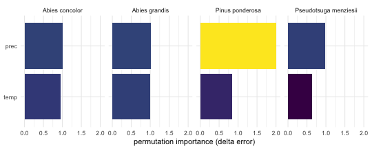
Each species leans on a different climate driver; the importances are learned per species, not shared.
Response to size and light: did the network recover the mechanistic form?
The point of a hybrid is to ask which functional form the neural network learned and how it compares to the mechanistic function it replaced. Here the two agree on the structural responses that are well constrained by the data: growth declines with tree size and increases with light availability for every species, and the network recovered both shapes without being given the functional form. That agreement is the useful result; it says the mechanistic size-and-light response was a reasonable choice, and that a flexible network, free to do anything, reproduces it. The remaining gaps between the curves are small next to the noise in the rate itself.
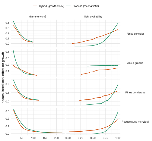
Each curve spans only the range its own model actually simulates (ALE never extrapolates), so where the process and hybrid cover different ranges, as for Abies grandis light, the two models simply place that species in different conditions; the mismatch is information, not an artefact.
sessionInfo()
#> R version 4.5.0 (2025-04-11)
#> Platform: aarch64-apple-darwin20
#> Running under: macOS 26.5.1
#>
#> Matrix products: default
#> BLAS:   /Library/Frameworks/R.framework/Versions/4.5-arm64/Resources/lib/libRblas.0.dylib
#> LAPACK: /Library/Frameworks/R.framework/Versions/4.5-arm64/Resources/lib/libRlapack.dylib;  LAPACK version 3.12.1
#>
#> locale:
#> [1] C
#>
#> time zone: Europe/Berlin
#> tzcode source: internal
#>
#> attached base packages:
#> [1] stats     graphics  grDevices utils     datasets  methods   base
#>
#> other attached packages:
#> [1] ggplot2_3.5.2     data.table_1.17.8 torch_0.15.1      FINN_0.1.0
#>
#> loaded via a namespace (and not attached):
#>  [1] Matrix_1.7-3       bit_4.6.0          gtable_0.3.6       dplyr_1.1.4
#>  [5] compiler_4.5.0     tidyselect_1.2.1   Rcpp_1.1.0         callr_3.7.6
#>  [9] splines_4.5.0      scales_1.4.0       lattice_0.22-6     R6_2.6.1
#> [13] labeling_0.4.3     generics_0.1.4     knitr_1.50         tibble_3.3.0
#> [17] pillar_1.11.0      RColorBrewer_1.1-3 rlang_1.2.0        xfun_0.57
#> [21] bit64_4.6.0-1      viridisLite_0.4.2  cli_3.6.6          withr_3.0.2
#> [25] magrittr_2.0.3     mgcv_1.9-1         ps_1.9.1           grid_4.5.0
#> [29] processx_3.8.6     lifecycle_1.0.5    nlme_3.1-168       coro_1.1.0
#> [33] vctrs_0.6.5        evaluate_1.0.5     glue_1.8.0         farver_2.1.2
#> [37] abind_1.4-8        tools_4.5.0        pkgconfig_2.0.3